Dylan Strome is tearing it up for the Chicago Blackhawks after putting up paltry numbers the last two seasons for the Arizona Coyotes, the team that drafted him third overall in 2015. Eric Staal experienced a career renaissance with the Minnesota Wild in 2016-17 and 2017-18, and this season to a lesser degree, after many thought his days of stardom were finished with the Carolina Hurricanes. Andrew Ladd and Brent Seabrook have seen their statistics take a large nosedive after receiving large contracts.
With all this in mind, the Coyotes and Hurricanes might be rethinking their decisions to give up on the two former players, while the New York Islanders and Blackhawks might be rethinking their signing of the latter two players. Wouldn’t it be nice if your team’s general manager could predict the future?
Dylan Strome’s Advanced Stats Hinted at His Turnaround
I actually became interested in this topic after I noticed Strome’s turnaround in Chicago, and I wondered exactly what happened. I went to moneypuck.com to look at some of his underlying stats to see if I could identify any trends. Granted, the information available for him from prior seasons is a small sample size and he very well could be a flash in the pan this season. However, the one thing I noticed was that he had a very high expected goals percentage (xG%) compared to his teammates.

Expected goals for is a metric that takes into account a player’s shots, the type of shots he is taking, and where he is taking those shots in an attempt to predict the amount of goals a player should be scoring for a given season. Expected goals for percentage takes the percentage of opportunities created for one’s team while said player is on the ice versus the percentage of opportunities created by the opposing team while said player is on the ice. It is an attempt to show whether a player is creating opportunities for themselves and their teammates.
Points Should Not Be the Only Measuring Stick
So with this very anecdotal evidence in Strome’s case, I set out to see if I could prove my hypothesis that xG% is a good predictor of a player’s future production. You can see below a chart showing the xG% for Staal. As you can see, Staal’s xG% remained high even in his least productive seasons in Carolina:

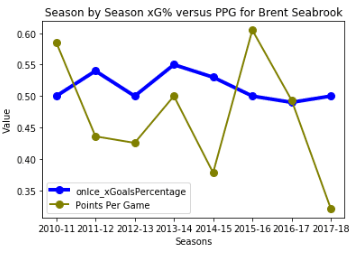
Meanwhile, as displayed in the below chart, Seabrook saw his xG% plummet the two seasons preceding his big contract pay day when he earned an eight-year extension worth an AAV of $6.85 million:
I think we fall into a trap of looking at points alone to judge a player’s career trajectory, especially for players who are young or relatively old. When a player is not progressing, we tend to think they are stalling in their development. For 30-plus year old stars, a dip in points tends to make us think they are on the decline. In both cases, fans, the media and even teams themselves are wrong all the time. I believe xG% is a helpful predictor for a player’s future productivity!
Expected Goals Can Help Us Predict Future Production
Using data from 2010 to 2018 from moneypuck.com, I ran a linear regression, which in statistics is an attempt to model a given dependent variable, in our case future points per game, based on independent variables, in our case the prior season’s xG% and points per game. I won’t bore you with too many details, but I have included a regression output below:
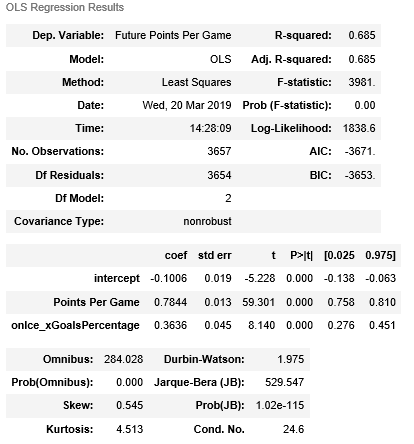
The key thing to note here is the R-squared number, which is a statistic meant to describe how much of the variation we see in our dependent variable can be described by our independent variables. Here we have an R-squared of 0.685, which means that nearly 70 percent of a player’s points per game in a season can be explained by our two variables. Both of our variables are statistically significant, meaning that they do have some effect on our dependent variable.
What is really fascinating is the coefficient for each of our variables. A coefficient shows the impact of a given variable on the dependent variable. In this instance, the coefficient for xG% is 0.3636, while the coefficient for points per game is 0.7844. This means that for every one percent change in xG% or points per game, you can expect to see a change of 0.3636% and 0.7844%, respectively, holding all other variables constant.
What this means is that we can come up with a prediction for a player’s points per game in the future based on both their xG% and their points per game in a given season. This can be shown in the following equation:
Future Points Per Game = -0.1006 +0.7844Points Per Game + 0.3636xG%
Teams Must Optimize Personnel Decisions Given Salary Cap Constraints
Take note that this equation is not a perfect indicator, especially at the highest levels of point scoring. However, I think we have enough evidence that a team should take both points per game and xG% into account before making decisions on signings or trades.
In the salary cap era, teams have to avoid making mistakes when signing or trading players. By using this model, teams can optimize their roster decisions. Maybe Strome would still be a Coyote if Arizona had done this analysis.
Free Newsletter
Get Advanced Stats coverage delivered to your inbox
In-depth analysis, breaking news, and insider takes - free.
Subscribe Free →